Classical Controllers (P, I, D)

In the previous post, we discussed the configuration of control systems. In this post, we will discuss the common types of controllers used in classical control systems.

Controllers

Every plant has certain characteristics and will behave a certain way when provided a unit step input. For example, the plant,

\begin{equation} \frac{Y(s)}{R(s)} = \frac{0.5}{0.1s + 1} \label{eqn:example_eq} \end{equation}

will have a steady state value of \(0.5\) (because \(K=0.5\)) for unit step input.

If, instead, we want to have a steady state value of \(1\) for the same unit step input, we can’t always change the plant itself. Therefore, we use a controller instead to “control” the output of the system. The controller is placed in cascade (in series) with the plant as shown below.

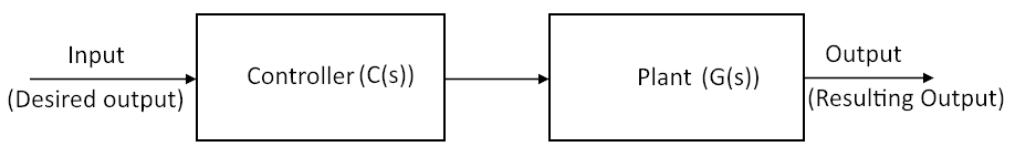
Controller and plant in open-loop configuration.
Figure 1: Controller and plant in an open-loop configuration.

To change the system in Equation \ref{eqn:example_eq}, so that the output is \(1\) when input is a unit step function, we can multiply the plant with \(2\). The controller, therefore, is just a constant gain of value \(2\). This type of controller is called a “Proportional controller”, and is the simplest type of controller that can be used.

Proportional \((P)\) controller

As mentioned before, \(P\) controller is the simplest type of controller that can be used. The output of a Proportional controller is proportional to the input of the controller. It is just a gain (can be positive or negative and can be a fraction) that is multiplied by the plant to modify its system response. A real-world example would be the use of an amplifier to amplify the sound from a speaker by a fixed amount. Figure 2 shows the output of the system in Equation \ref{eqn:example_eq} in open-loop configuration. The steady state value is \(0.5\) as expected.

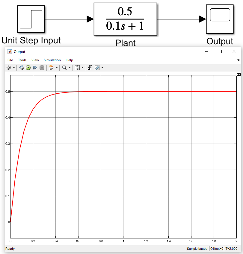
Figure 2: Unit step response of the system.

However, when a Proportional controller with a gain of \(2\) is used, the steady state value changes to \(1\), as shown in Figure 3.

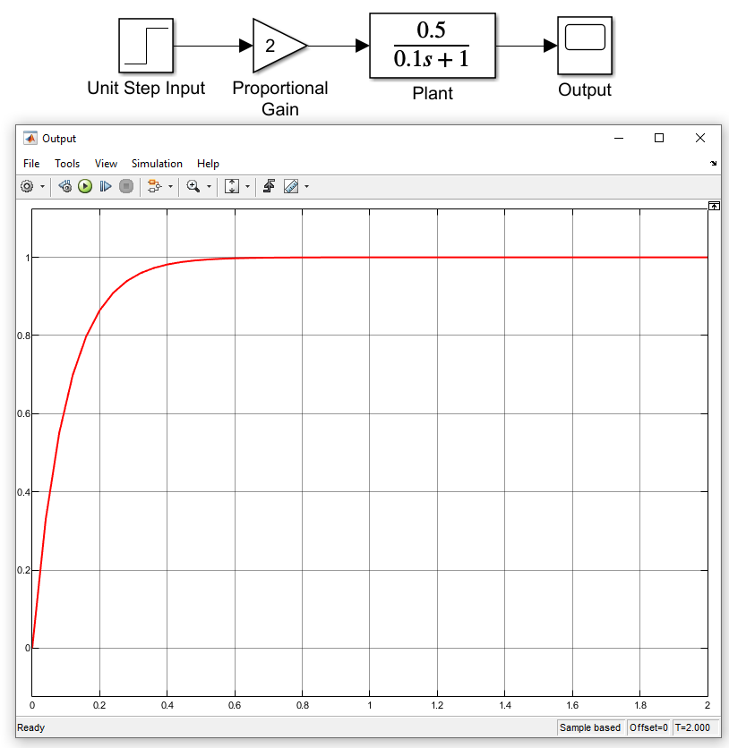
Figure 3: Unit step response of the system with Proportional controller.

Integral \((I)\) controller

The output of an Integral controller is proportional to the integral of the input to the controller. In terms of a closed-loop system, as shown in Figure 4, the output of the \(I\) controller is the integral of the error term. Integral controllers are useful because they cause the system to have zero steady state error. Integral controllers will also increase the type of a system i.e., a first-order system will become a second-order system, and a second-order system will become a third-order system, and so on.

Figure 4: Closed-loop system with a PI controller.

Derivative \((D)\) controller

The output of a Derivative controller is proportional to the derivative of the input to the controller. In terms of a closed-loop system, the output of the \(D\) controller is the derivative of the error term. Derivative controllers are never used on their own and are usually paired with a \(P\) controller to make a \(PD\) controller, or a \(PI\) controller to make a \(PID\) controller. Derivative controllers are useful because they act as a dampener on the control effort. If the system is oscillating a lot, then the introduction of a derivative controller can damp those oscillations.

Example of a PI controller

Let us suppose that the plant we need to control is a first-order system with the following transfer function,

\[\frac{Y(s)}{R(s)} = \frac{2}{4s + 2}\]

We can calculate \(K=1\) and \(\tau=2\) as follows:

\[\frac{Y(s)}{R(s)} = \frac{2}{4s + 2} = \frac{\frac{2}{2}}{\frac{4s}{2} + \frac{2}{2}} = \frac{1}{2s + 1}\]

The closed-loop unit step response is shown in Figure 5.

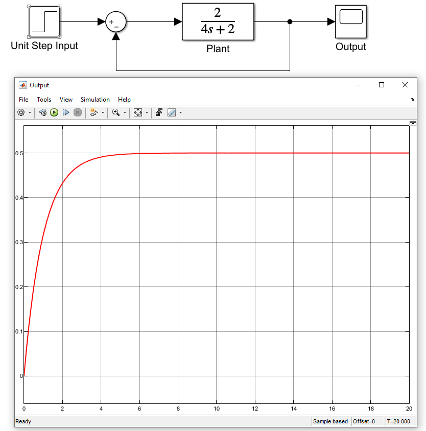
Figure 5: The closed-loop unit step response of the system.

As you can see, the system reaches a steady state around \(6\)s. But what if you want the system to reach a steady state at or less than \(2\)s? And the maximum overshoot you can tolerate is \(5\%\)? These are called system requirements and are chosen by you, or are given to you by someone who wants you to design the controller. Let’s design a PI controller that will give us the desired performance.

The system requirements are,

Percentage Overshoot \((PO) \leq 5\%\)
\(2\%\) Settling time \((t_s) \leq 3s\)

First of all, we need to create a block diagram of the system. The block diagram for a PI controller is shown in Figure 6.

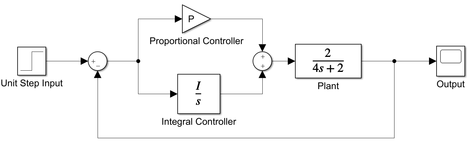
Figure 6: The PI controller with the plant.

This block diagram can be reduced in the following steps to get the transfer function in terms of variables \(P\) and \(I\) which are the proportional and integral gains respectively.

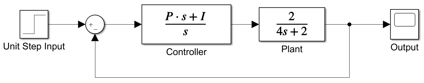
Figure 7: Step 1 of reducing the block diagram.

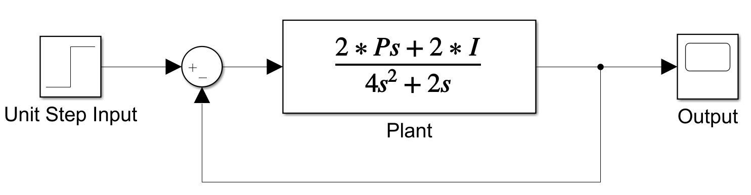
Figure 8: Step 2 of reducing the block diagram.

Using the closed-loop formula,

\[\frac{G}{1+GH}\]

where \(G = \frac{2(Ps+I)}{4s^2 + 2s}\), and \(H=1\), the transfer function is,

\[\frac{Y(s)}{R(s)} = \frac{2(Ps+I)}{4s^2 + 2s + 2(Ps+I)}\] \[\frac{Y(s)}{R(s)} = \frac{2(Ps+I)}{4s^2 + 2s (1 + P) + 2I}\]

Divide the numerator and the denominator by \(4\) to make the coefficient of the highest power of \(s\) in the denominator equal to \(1\) (This will come in handy later).

\begin{equation} \frac{Y(s)}{R(s)} = \frac{0.5(Ps+I)}{s^2 + 0.5s (1 + P) + 0.5I} \label{eqn:calculatedTF} \end{equation}

Now that we have the transfer function in terms of \(P\) and \(I\), we need to calculate the desired \(\zeta\) and \(\omega_n\) of the system. These can be computed based on the system requirements.

Calculating \(\zeta\)

\[\zeta = \sqrt{ \frac{\ln^2{(\frac{PO}{100})}} {\pi^2 + \ln^2{(\frac{PO}{100})}} }\]

Since \(PO \leq 5\%\),

\[\zeta \geq \sqrt{ \frac{\ln^2{(\frac{5}{100})}} {\pi^2 + \ln^2{(\frac{5}{100})}} }\] \[\zeta \geq 0.6901\]

Calculating \(\omega_n\)

\[t_s \geq \frac{-\ln{(0.02)}}{\omega_n \zeta}\]

Since \(2\% (t_s \leq 3s\), and the calculated \(\zeta \geq 0.6901\),

\[\omega_n \geq \frac{-\ln{(0.02)}}{t_s \zeta}\] \[\omega_n \geq \frac{-\ln{(0.02)}}{(3)(0.6901)}\] \[\omega_n \geq 1.89 \text{ rad/s}\]

Putting all the pieces together

The transfer function we calculated is for a second-order system. We previously mentioned that the transfer function for a second-order system is of the general form,

\[\frac{Y(s)}{R(s)} = \frac{{\omega_n}^2}{s^2 + 2 \omega_n \zeta s + {\omega_n}^2}\]

Take the denominator of the general form and populate it with the calculated \(\zeta\) and \(\omega_n\) values.

\[s^2 + 2(1.89)(0.6901) s + {(1.89)}^2\]

Now make this equal to the denominator of the transfer function you derived from the block diagram (Equation \ref{eqn:calculatedTF}).

\[s^2 + 2(1.89)(0.6901) s + {(1.89)}^2 = s^2 + 0.5s (1 + P) + 0.5I\]

Now match the \(s\) terms and solve for the unknowns

Finding \(P\),

\[2(1.89)(0.6901) s = 0.5s (1 + P)\] \[5.217 = 1 + P\] \[P = 4.214\]

Finding \(I\),

\[1.89^2 = 0.5I\] \[I = 7.144\]

Putting these values of \(P\) and \(I\) in the transfer function, we get the following unit-step response,

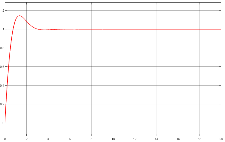
Figure 9: Incorrect result after using the calculated PI gains.

The settling time is below \(3\)s which fulfills the \(2\%\) requirement, however, the percentage overshoot is more than \(5\%\). This is because the calculation only provides a close guess of the required PI gains. After performing the calculation, the gains need to be manually tuned to get the desired system response. Upon manually tuning the \(P\) gain to \(8\), we get the desired system response as shown in Figure 10. The \(I\) gain was not changed.

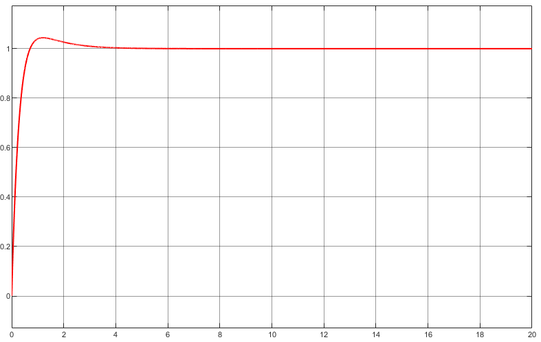
Figure 10: Correct result after tuning the PI gains.

Note: The gains can also be manually tuned without performing the calculation. However, the time it takes to get the desired gains will vary. You might be able to find the gains very quickly, or it might take a very long time. Therefore, performing the calculations gives you a good starting guess and you can start tuning the gains from there.

PID controllers and third-order systems

The calculation of a third-order system follows in a similar way as a second-order system with a small difference. The block diagram of a plant with a PID controller is shown below.

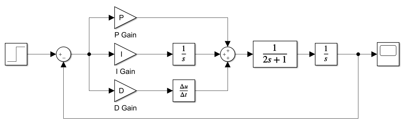
Figure 11: The PID controller with the plant.

Calculating the PID gains

The block diagram shown in Figure 11 can be reduced similarly as shown for the PI controller but with three variables i.e., \(P\), \(I\), and \(D\) gains. If the plant is a second-order system (as shown in Figure 11), then the overall transfer function will result in a third-order system. Since we only know how to solve for a second-order system, we do a little trick. The transfer function of Figure 11 is shown below:

\[\frac{Y(s)}{R(s)} = \frac{\frac{Ds^2+Ps+I}{2}}{s^3 + s^2\frac{(1+D)}{2} + s\frac{P}{2} + \frac{I}{2}}\]

Since we know that a third-order system has 3 poles, we choose one of the poles and then calculate the rest of the two poles using the system requirements (Percentage overshoot and Settling time).

Choosing the third pole

To explain the choice of a pole, let us take an example transfer function and see how its poles and zeros (the roots of the denominator and numerator, respectively) look like in the s-plane. In the figure below, the root locus for a third-order system with the following transfer function is shown:

\[\frac{Y(s)}{R(s)} = \frac{s+1}{s^3 + 57s^2 + 360s + 500}\]

The system has poles at \(-2\), \(-5\), and \(-50\) and a zero at \(-1\).

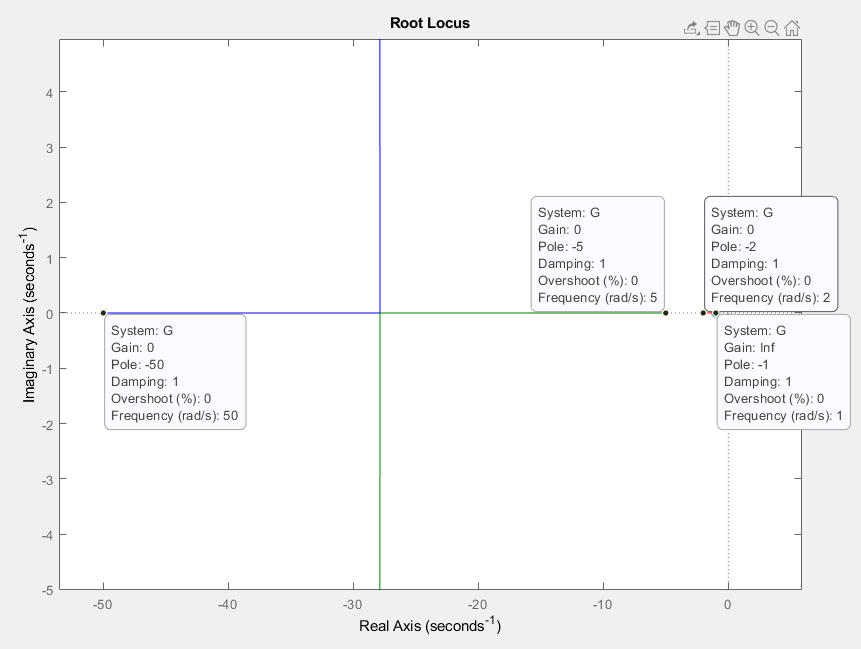
Figure 12: Root locus of a third-order system with poles at \(-2\), \(-5\), and \(-50\) and a zero at \(-1\).

Any third-order system behaves like a second-order system if one of the three poles of the system (the order of the system tells how many poles it has) is to the far left of the imaginary axis.

In the example shown in Figure 12, the third pole at \(-50\) is very far to the left of the imaginary axis and therefore, has minimal effect on the system response. The nearer a pole is to the imaginary axis, the more impact it has on the system response.

With this knowledge, and the knowledge that the characteristic equation of a second-order system is as follows,

\[s^2 + 2\omega_n \zeta s + {\omega_n}^2\]

we can write down the characteristic equation of the third-order system. We can imagine a third pole more than \(5\) times that of the other two poles and place it at the far left of the imaginary axis. The resulting equation is,

\[(s-\alpha)(s^2 + 2\omega_n \zeta s + {\omega_n}^2)\]

where \(\alpha\) is the pole that we choose. We can choose an arbitrarily large negative value such as \(-100\), or we can choose \(\alpha\) to be \(-\omega\zeta\). In either case, we have a third pole that will not affect the system response too much and will allow us to approximate the third-order system as a second-order system. After this step, the calculation is similar to that of a system with a PI controller.

System requirements and calculating the PID gains

The system requirements to design the PID controller for the system shown in Figure 15 are,

Percentage Overshoot \((PO) \leq 5\%\)
\(2\%\) Settling time \((t_s) \leq 3s\)

Based on these system requirements, the calculations follow from the PI controller example in part 6.

The resultant \(\zeta \geq 0.6901\)
The resultant \(\omega_n \geq 1.89 \text{ rad/s}\)

We can choose the third pole \(\alpha = -100\) and put the \(\zeta\) and \(\omega_n\) values calculated above, in the third-order characteristic equation below,

\[(s-\alpha)(s^2 + 2\omega_n \zeta s + {\omega_n}^2)\] \[(s+100)(s^2 + 2(1.89)(0.6901) s + {(1.89)}^2)\] \[(s+100)(s^2 + 2.609 s + 3.572)\] \[s^3 + 2.609 s^2 + 3.572s + 100s^2 + 260.9s + 357.2\] \[s^3 + 102.609 s^2 + 364.472s + 357.2\]

Once we have this equation, we can equate it to the denominator of the transfer function we found for the system in Figure 11.

\[s^3 + 102.609 s^2 + 364.472s + 357.2 = s^3 + s^2\frac{(1+D)}{2} + s\frac{P}{2} + \frac{I}{2}\] \[102.609s^2 = \frac{1+D}{2}s^2\] \[D = 204.218\] \[364.472s = \frac{P}{2}s\] \[P = 728.944\] \[357.2 = \frac{I}{2}\] \[I = 714.4\]

Since we are approximating a second-order system behavior from a third-order system, after calculating the PID gains, we might need to manually tune them to get the desired system response.