System Configuration, Transfer Function, Laplace Transform, and System Order.

System configuration

A plant (also referred to as a process) in control theory is something that receives an input and after processing it, gives a specific output. A plant is usually denoted by \(G\). A system is composed of other smaller sub-systems such as plants and controllers etc. A system can have open-loop and closed-loop configurations.

Open-loop system

The figure below shows a system in an open-loop configuration. An open-loop system receives an input and gives back an output. However, the output does not influence the input in any way.

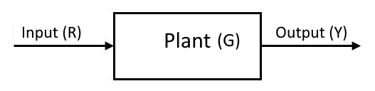
Figure 1: An open-loop system

For example, a DC motor in an open-loop configuration takes voltage \((V)\) as an input and gives angular velocity \((\omega)\) as an output. You can change \(V\) to change \(\omega\) but the change in \(\omega\) does not influence \(V\). Figure 2 shows an example of a DC motor receiving an input and giving an output.

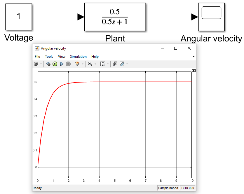
Figure 2: DC motor in open loop configuration and the resulting output when a constant 1 V input is given

Closed-Loop System

In a closed-loop system, a fraction of the output is fed back to the input and either added to or subtracted from the input. If the output is added, we call this a positive feedback system. If the output is subtracted from the input, we call it a negative feedback system. For system robustness, we typically use a negative feedback control. The feedback gain is denoted by \(H\). If there is no \(H\) in the feedback loop, then the value of \(H\) is considered to be 1 and the entire output is fed back to the input (for the sake of clarity, \(G(s)\) and \(H(s)\) are shown as \(G\) and \(H\)).

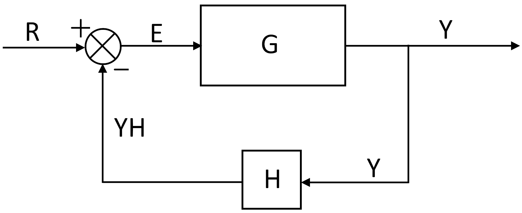
Figure 3: A closed-loop system with plant \(G(s)\) and feedback \(H(s)\).

Here, \(R\) is the input, \(Y\) is the output, \(E\) is the error (difference between input and the feedback value)

\[E(s) = R(s) - Y(s)H(s)\]

Transfer Function

A Transfer Function is the ratio of the output of a system to the input of a system in the Laplace domain, considering its initial conditions and equilibrium point to be zero.

For the Block diagram in Figure 3, the transfer function is calculated as follows (for the sake of clarity, \((s)\) is omitted from the equations. All terms are in the Laplace domain):

\[Y = GE\]

Substituting \(E = R(s) - Y(s)H(s)\) in the equation above, we get,

\[Y = G\left(R - YH\right)\] \[Y = GR - GYH\] \[Y + GYH = GR\] \[Y(1 + GH) = GR\] \[Y = \frac{GR}{(1 + GH)}\]

Finally, the transfer function is:

\[\frac{\text{Output}}{\text{Input}} = \frac{Y(s)}{R(s)} = \frac{G}{1 + GH}\]

Laplace Transform

The transfer function of a given system can be computed by first deriving its differential equations. Then convert those time domain equations into the Laplace domain by applying the Laplace transform. The third step is to find the ratio of the output to the input and that is the transfer function of that particular system.

For example, for a spring mass damper system with an input force \(f(t)\), mass \((m)\), damping coefficient \((d)\), and spring constant \((k)\), the differential equation is as follows:

\[m\ddot{x}(t) + d\dot{x}(t) + kx(t) = f(t)\]

To take the Laplace transform of a quantity that is a function of time \(t\) when the initial condition is 0, the following transformation can be used.

\[x(t) \text{ becomes } X(s)\] \[\dot{x}(t) \text{ becomes } sX(s)\] \[\ddot{x}(t) \text{ becomes } s^2X(s)\]

and so on.

With this information, we can convert the equation above to the Laplace domain using the Laplace transform.

\[m\ddot{x}(t) + d\dot{x}(t) + kx(t) = f(t)\]

becomes

\[ms^2X(s) + dsX(s) + kX(s) = F(s)\]

Now for the last part, we can find the ratio of output \(X(s)\) to the input \(F(s)\).

\[X(s)(ms^2 + ds + k) = F(s)\] \[\frac{X(s)}{F(s)} = \frac{1}{ms^2 + ds + k}\]

Congratulations, now you know how to compute a transfer function!

Note: This is a simplification of the Laplace transform calculation and is ONLY valid if the initial conditions are considered to be 0. The good news is that is all we need for the course. The actual Laplace transform looks like this,

\[\mathcal{L}\{f\}(s) = \int_{0}^{\infty} f(t) e^{-st} dt\]

System Order

The order of a system depends on the highest order of the derivative in the differential equation of a system. For a system with a differential equation,

\[\ddot{x}(t) + a\dot{x}(t) = b\]

The highest order of derivative is 2 (you have a double derivative in the equation). Therefore, it is a \(2^{nd}\) order system.

In the Laplace domain, the order of the system can be determined by looking at the highest power of the \(s\) term. In the following transfer function,

\[\frac{Y(s)}{R(s)} = \frac{s + 1}{s^3 + 2s^2 + 6s + 4}\]

the highest power of \(s\) is 3, therefore, it is a \(3^{rd}\) order system.

System response

The system response refers to the system output when a known input is given to the system. Typically, a unit step function is used as an input and is shown below:

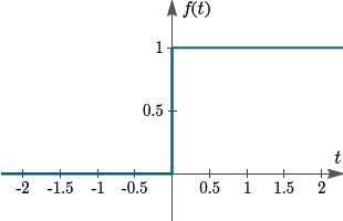
Figure 4: The unit step function.

The unit step function has a value of 0 before time \(t = 0\), and a value of 1 onward. This is used as an input because it is the simplest input possible and is used as a standard to compare the outputs. Other inputs include an impulse function, ramp function, etc.

\(1^{st}\) order systems

A first-order system has a transfer function of the following form:

\[\frac{Y(s)}{R(s)} = \frac{K}{\tau s + 1}\]

where \(K\) is called the DC gain and \(\tau\) is the time constant of the system.

Figure 5 shows the unit step response of a \(1^{st}\) order system, and can be explained by the following equation in the time domain,

\[y(t) = (y(0) - y_{\infty})e^{(- \frac{t}{\tau})} + y_{\infty}\]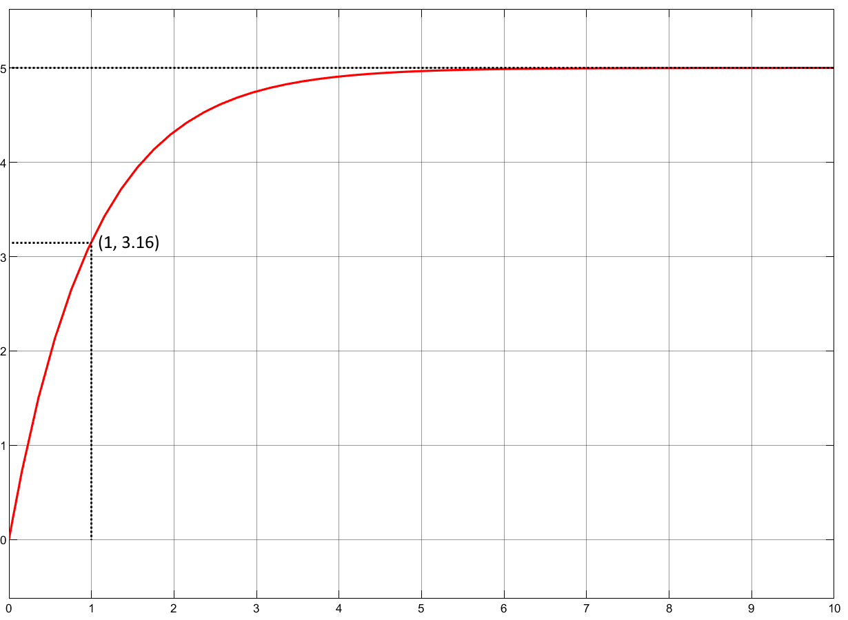

First order system with K and tau calculation.
Figure 5: First order system with \(K\) and \(\tau\) calculation.

Transient and Steady state

The transient state of a step response is when the output changes at every time instant. The steady state of a system is when the output reaches a steady value and does not change at every time instant.

In Figure 5, the transient state starts from time \(t = 0\) and ends at \(t = 6\). The steady state starts when the transient state ends and goes on until \(t = \infty\).

In closed-loop systems, if the steady-state output is not the same as the input, then the difference between the input and the output is called steady state error.

\(K\) and \(\tau\) calculation

The transfer function of a first-order system can be calculated from its step response graph. \(K\) is the DC gain of the system and is equal to the steady state value of the system. In Figure 5, the steady state value is 5, therefore \(K = 5\). To calculate \(\tau\), find the time at which the output reaches 63.2% of \(K\). Since \(K = 5\) in Figure 5, 63.2% of \(K\) is 3.16. The time at \(y = 3.16\) is 1s. Therefore, \(\tau = 1\)s. Using this information, we can find the transfer function of the system in Figure 5 to be,

\[\frac{Y(s)}{R(s)} = \frac{K}{\tau s + 1} = \frac{5}{s + 1}\]

\(2^{nd}\) order systems

A second order system has a transfer function of the following form:

\[\frac{Y(s)}{R(s)} = \frac{{\omega_n}^2}{s^2 + 2 \omega_n \zeta s + {\omega_n}^2}\]

where \(\omega_n\) is the natural frequency and \(\zeta\) is the damping ratio of the system.

Figure 6 shows the unit step response of a \(2^{nd}\) order system and the effect of changing the damping ratio \((\zeta)\) on the system response.

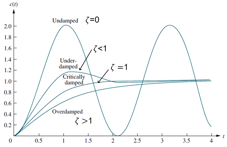
Effect of damping ratio zeta) on the unit step response of a second-order system.
Figure 6: Effect of damping ratio \(\zeta\) on the unit step response of a second-order system.

For a stable system, \(\zeta\) can have four different states. These states are discussed below.

Undamped system \((\zeta = 0)\)

When a system is undamped, it oscillates for time \(t = \infty\) because there is no damping in the system. Therefore, the system is stable, i.e., the output never diverges (it is bounded), and it never reaches a steady state.

Under-damped system \((\zeta < 1)\)

When a system is under-damped, the output initially overshoots the input (desired) value and then after several oscillations, reaches a steady state. The oscillations are a result of the under-damping of the system and some oscillation in the system is usually acceptable. However, this also depends on the system in question. For some critical systems, we do not want any oscillations, for others, we do not care that much about minor oscillations.

Critically damped system \((\zeta = 1)\)

When a system is critically damped, the output reaches a steady state without any overshoot. However, any minor reduction in the damping ratio (0.999 for example) will cause an overshoot in the output.

Over-damped system \((\zeta > 1)\)

A system is over-damped when it reaches a steady state without any oscillations and a small decrease in the damping ratio doesn’t cause any overshoot/oscillations.

\(\zeta\) and \(\omega_n\) calculation

To calculate \(\zeta\) and \(\omega_n\), we need to know the following two pieces of information:

Percentage Overshoot \((PO)\) - The percentage by which the output overshot the input value
Settling time \((t_s)\) - the time it took for the system to reach steady state

Note: Since the system oscillates for quite a while very close to the steady state, we take settling time as the time when the output is 2% of the steady state (when output is within the 2% range of the steady state. For example, if the steady state is 1, the settling time can be the time it takes for the output to reach 1.02 or 0.98 or any value in between, whichever comes first).

As an example, we will consider a system with 5% overshoot \((PO)\) and a settling time \((t_s)\) of 3s.

Damping ratio \((\zeta)\) can be calculated as follows:

\[\zeta = \sqrt{ \frac{\ln^2{(\frac{PO}{100})}} {\pi^2 + \ln^2{(\frac{PO}{100})}} }\] \[\zeta = \sqrt{ \frac{\ln^2{(\frac{5}{100})}} {\pi^2 + \ln^2{(\frac{5}{100})}} }\] \[\zeta = 0.6901\]

Natural frequency \((\omega_n)\) can be calculated as follows:

\[t_s = \frac{-\ln{(0.02)}}{\omega_n \zeta}\] \[\omega_n = \frac{-\ln{(0.02)}}{t_s \zeta}\] \[\omega_n = \frac{-\ln{(0.02)}}{(3)(0.6901)}\] \[\omega_n = 1.89 \text{ rad/s}\]

Note: The 0.02 in -\(\ln{(0.02)}\) refers to the 2% settling time. If you want to consider a 1% settling time, just change the value to 0.01.

In the next post, we will discuss the different types of controllers and their effects on the system response.