Simulating a Swarm of Robots in Gazebo
In this project, I simulated a swarm of robots in Gazebo. The robots were controlled using a decentralized control algorithm that allowed them to move in a formation while avoiding obstacles.
Introduction
Here I elaborate on the steps taken and approach adopted to simulate a swarm of robots and discuss an attempt to take the robots from the home position to the goal. I report the successes and the failures during this project and suggest solutions that might improve the simulation and give better results.
Formation
The robots start with the following initial formation
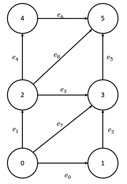
Figure 1: Swarm formation.
The length of the horizontal edges is 0.75 m. The length of the vertical edges is 1 m. The leader robot \((r_0)\) can move freely, whereas the rest of the robots react to its movement and try to maintain formation.
The approach to maintain formation is to keep a balance between the Laplacian and the edge length \((z_{des})\) values. The robots start to move when the sum of the Laplacian values and the corresponding \(z_{des}\) value is non-zero. Their sole purpose during the simulation is to keep the difference zero and it is due to this constraint, that they can follow \(r_0\) and maintain formation. This can be shown as the following equation,
\[v_{wheel} = (d_i - z_{des}) \times k\]where \(d_i\) is the distance between the robot and its \(i^{th}\) neighbor, \(z_{des}\) is the desired distance between the robots, and \(k\) is the gain value.
Before starting the simulation, the robot heading, and current wheel encoder values are saved inside the robot object. For \(r_0\), additional data pertaining to the current time, next waypoint index, and the time delay to change direction are saved as well. The figure below shows the initialization sequence.
Navigation
The project did not consider path planning and the robots move by assuming that there are no obstacles in their way. Attempts were made earlier during the project to build an obstacle avoidance system, but those pursuits were eventually abandoned to focus on the formation control part of the project which held the most importance. This was primarily done because the controller used to drive each robot is not very efficient and the robot must stop in its tracks every time it wants to change its direction. This stop-and-go behavior leads to errors in the estimation of the obstacle position and since the “changing direction” and the “moving forward” are two distinct sequences, when the robot is moving forward, it cannot change direction even though it knows that there is an obstacle in front of it.
The current approach to navigation is that \(r_0\) is given distinct waypoints to go to and the rest of the robots follow it to maintain formation. The fact that the entire map is a huge grid was not left unnoticed and this was utilized to make \(r_0\) move in horizontal, vertical, and diagonal lines, to make the navigation as simple as it can be. \(r_0\) moves very slowly so that other robots have enough time to catch up, and waits for a few seconds when it reaches a waypoint to change direction and wait for other robots.
Here are a couple of videos of the simulation:
Enjoy Reading This Article?
Here are some more articles you might like to read next: